Monte Carlo Simulations
for roadmap estimation
Monte Carlo methods are a family of algorithms that employ repeated random sampling to build a model of probable outcomes: effectively, it is the mathematics of uncertainty. Monte Carlo math was developed for modeling the behavior of neutrons during atomic decay, a problem where deterministic algorithms proved inadequate. Estimating software isn’t as complex as nuclear physics, but that’s small comfort when it’s up to us to ask for the right amount of resources to build a product. Monte Carlo Simulations allow us to replace the proverbial wild ass guess with manageable probabilities.

Probabilistic Modeling
In contrast to deterministic models, Monte Carlo simulations turn things around to model probable outcomes based on what we do know. We can use Monte Carlo simulations when the complexity of what we’re trying to model gets to be more than we can manage. As long as we can decompose the problem into questions that we can reason about independently, and express our uncertainty about those questions in ranges, then we can model the work to infer probable outcomes. Our goal is to support decisions with better information.
You don’t have to learn Monte Carlo math to use it in a spreadsheet model, any more than you have to work out the math of electricity to use your laptop.
How to Get Started
The inputs for our Monte Carlo model are range value estimates from individual components of work, which we’ve broken down to the point where we can reason about them. A range value estimate expresses our degree of certainty about the effort required to accomplish the work. A small range indicates greater certainty, in contrast to a wide range, which indicates greater uncertainty.
Our model inputs are an array of independently estimated components of work. The range estimates that constitute our model inputs are easy to change whenever new information reduces (or increases) our uncertainty. When we update inputs based on new information, then our model automatically recalculates to reflect how the new information impacts probable outcomes.
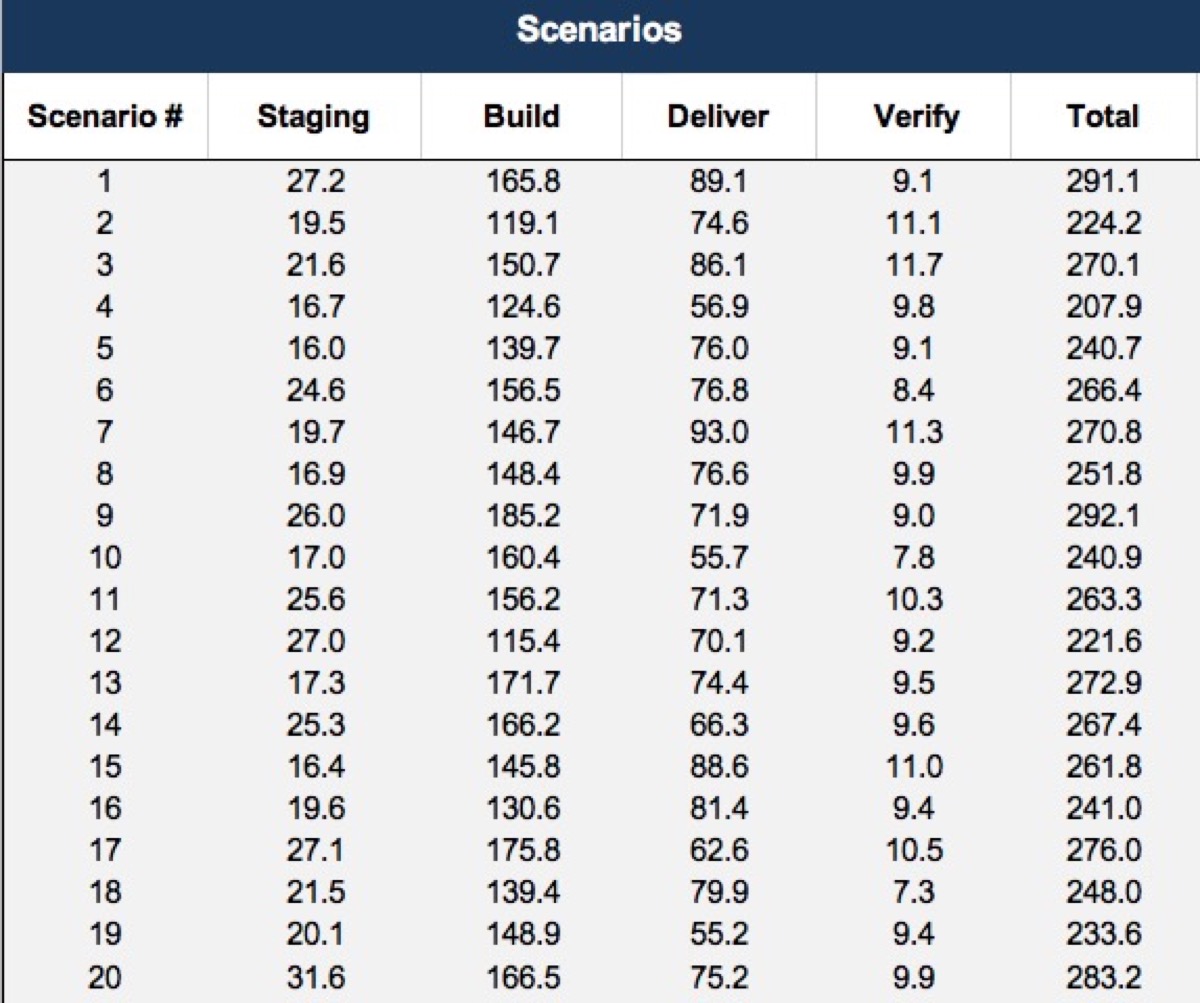
For example if we’re asked to make a high-level estimate for a project that we don’t know a whole lot about yet, we might break the work down into components of Staging, Build, Delivery and Verification, and ask various teams for range estimates, likely just parametric estimates, based on comparison with previous projects.
Say they come back with these estimates:
The first thing we do to build our spreadsheet simulation is to provide our range estimate inputs and calculate the mean of each. The mean can be calculated in a couple of ways, but for our purposes, we can use the Excel Average() function, with the low and high values of the estimate as parameters. For example, if we have a dollar estimate with a low of 120k and high of 180k hours, the mean is $150k.
Here’s our estimate inputs with the mean:
Constructing a Scenario
Once we have the mean of a range estimate, then we can generate a randomized value like this:
=NORMINV(RAND(),mean,(low-high)/distribution)
Where mean, low and high are tokens which refer to what would be absolute cell addresses, pointing to the corresponding values for a single range input. To short-circuit what could be a very long discussion on the math of distributions, we’ll suggest 3.29 as the normal distribution.
That formula represents one cell in a scenario; A scenario is comprised of a set of cells with that formula, one for each of the component estimates inputs. Each cell is individually randomized. The sum of all the cells in the scenario is the roll-up of a scenario.
Once we build one scenario, we can reproduce it many times, say 10,000 rows, by copy and paste.
Distribution of Scenarios
The next component of the Monte Carlo is to distribute the results of the randomized rollups to an array of equal sized elements or bins. The first bin holds the lowest values from the randomized rollups, and the last bin holds the highest values. The exact number of bins you use isn’t essential, whatever works to allow us to make sense of the distribution. The number of scenarios that fall in each bin indicates the probability of an outcome in that range. There are some choices for how to make the distribution; a normal distribution would be an excellent place to start.
All that’s left now is to render the distribution as a histogram: a visualization of probable outcomes.
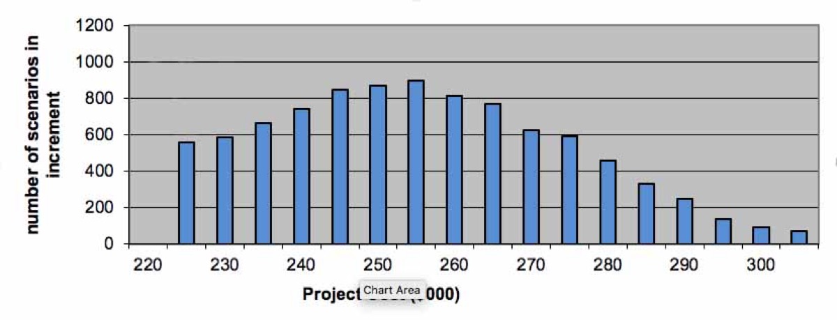
We’ve taken a problem that is too complex to reason about, broken it down to components of work which are independently estimated, and then visualized the probability of outcomes based on our range estimate inputs.

Let's agree to define productivity in terms of throughput. We can debate the meaning of productivity in terms of additional measurements of the business value of delivered work, but as Eliyahu Goldratt pointed out in his critique of the Balanced Scorecard, there is a virtue in simplicity. Throughput doesn’t answer all our questions about business value, but it is a sufficient metric for the context of evaluating the relationship of practices with productivity.